New release: Test any website or web app. No code needed.
Learn more
The 3D cluster view (3DCV) visualizes the similarity between cards as three-dimensional spatial relationships. Each point in the visualization represents an individual card. Cards that are closer together were more frequently sorted into the same category. The further apart that any two cards appear, the less frequently they were sorted together.
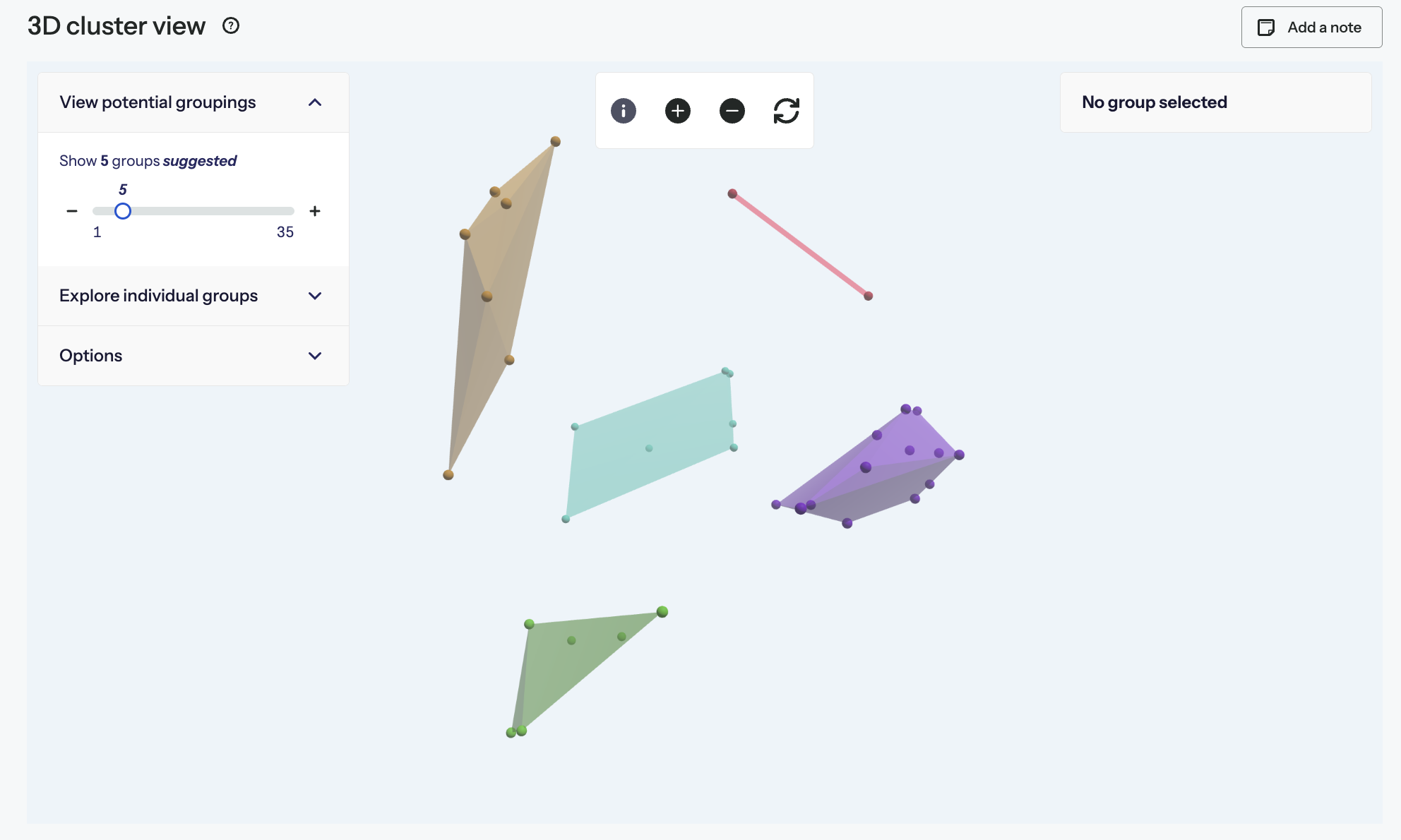
Polygons are shown over groups of cards that are clustered together. Each of these groups can be interpreted as a potential category within an information architecture. You’ll also see suggested category labels for each group. These are derived from looking at how many participants created similar categories to a particular group and comparing the most common labels that participants gave these categories. If you have standardized your users’ groups, the labels you have applied to the standardized groups will likely be suggested.
The 3DCV combines aspects of both the similarity matrix and the dendrograms by visualizing the similarity between cards and potential groupings of cards. The difference between 3DCV and these analysis approaches is that 3DCV provides a new perspective of card sort results by presenting these relationships in three-dimensional space.
The 3D Cluster view is a form of Multidimensional Scaling (MDS). MDS is a technique that translates a table of similarities between pairs of cards into a map where distances between the points match the similarities as much as possible. Similar cards are closer together, dissimilar cards are further apart.
Of course, the relative similarities between all of the cards in a sort do not exist on the same scale; it’s multidimensional. In our case, the distance matrix can be derived from the similarity matrix where each point in the dataset is an individual card. This means that a card sort with 50 cards would generate a 50 by 50 distance matrix, resulting in 50 dimensions (your brain is probably hurting at this point). The trick that MDS pulls off is to present these multitudes of dimensions in a simplified set of dimensions we can view – i.e. in 3D.
In more technical terms, it uses a function minimization algorithm that evaluates different configurations with the goal of maximizing the ‘goodness of fit’. All of those similarity pairings are presented as a set of points in 3D space that are close to, or distant from each other.
Having done this we have lots of dots in a 3D space. Now we want to see if we can spot any clustering groups in those dots.
We then use a hierarchical clustering method to separate the cards into a hierarchy of groups, similar to the structure of a dendrogram. Groups are divided in a way that ensures that the most similar cards are grouped together. Each level of the hierarchy corresponds to the number of groups displayed. At the top level there is one group containing all of the cards, at the second level there are two groups that together contain all of the cards, and so on.
The grouping slider on the 3D Cluster view changes the level of the hierarchy that is currently displayed.
Why are 8 groups (in this example) suggested? This is because the median number of categories that your users created was 8. If you remember, you can see that from the Overview tab.
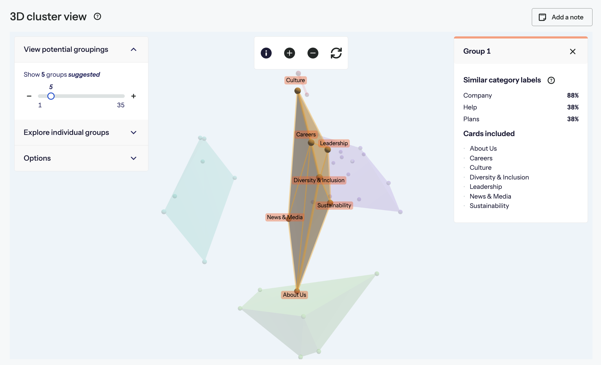
Clicking on a group will show you the cards within that group and also the category labels that are similar to the cluster. These labels are the ones that your users applied to groupings or that you applied when you standardized your users’ groupings.
Merging and splitting
Instead of navigating the hierarchy with the groupings slider, you can select a specific group and ‘split’ it into two. You typically might do this if you think it is too big or spans too great a distance between cards, or because you think this might present a better opportunity for the eventual hierarchy you are going to make.
You can also ‘merge’ clusters. When you ‘merge’, select a group and the algorithm will merge that group with the next-closest group.